The Truth is out There...in the Data.
When The X-Files revival was announced, my wife and I decided to catch up on the series before watching any of the new episodes. At the time, the entire catalog was available for streaming on Netflix. Thus, we began the long journey of watching over 200 episodes.
Sadly, the series was pulled from streaming before we could finish this endevour. Personally, I felt that the series really starting going downhill during season 7. Additionally, after David Duchovny left in season 8, it became almost painful to continue watching. Fox Mulder was replaced with the John Doggett character who just could not keep the show afloat. Surely the consenus of viewers must also have felt the same way.

After watching hours and hours of campy sci-fi, I wanted quality metrics on the show. The X-Files often featured guest writers and directors which caused the pace of the show to vary immensely. How did this variation in writers impact the quality of the show? The initial questions that I attempted to answer were the following:
- Which season of The X-Files had the hightest rating?
- Were “Monster of the Week” standalone episodes received better or worse than episodes based within the show’s overall narrative?
- Which writer of The X-Files wrote episodes with the highest ratings?
In order to answer these questions I needed data on each episode. I used Wikidata as my initial data source.
Wikidata is a free and open knowledge base that can be read and edited by both humans and machines.
Effectively, Wikidata is an indexing system that exposes this knowledge base through various APIs.
To grab data from Wikidata, I used the SPARQL query language.
This was my first time using SPARQL, but will not be my last. The syntax is still somewhat cryptic, however it provides access to a wealth of freely available data.
In SPARQL, variables are assigned following the SELECT statement with ?.
In the following query, I am defining 9 variables to be extracted from The Wikidata entity for the X-Files Q2744.
PREFIX wikibase: <http://wikiba.se/ontology#>
PREFIX schema: <http://schema.org/>
PREFIX wd: <http://www.wikidata.org/entity/>
PREFIX wdt: <http://www.wikidata.org/prop/direct/>
PREFIX p: <http://www.wikidata.org/prop/>
PREFIX pq: <http://www.wikidata.org/prop/qualifier/>

SELECT ?show ?episodeID ?showLabel ?season ?seasonNumber ?episode ?imdb ?episodeLabel ?url WHERE {
    BIND(wd:Q2744 as ?show) .
    ?season wdt:P361 ?show .
    ?episode wdt:P361 ?season .
    ?season p:P179 [
            pq:P1545 ?seasonNumber] .
    ?episode wdt:P345 ?imdb .
    ?episode wdt:P2364 ?episodeID.
    ?episode rdfs:label ?episodeLabel .

    ?url schema:about ?episode .
    ?url schema:inLanguage "en" .
    ?url schema:isPartOf <https://en.wikipedia.org/> .

    FILTER(langMatches(lang(?episodeLabel),"en"))
}
Variables are defined in the WHERE clause by binding them with schema P(Property) values.
?season wdt:P361 ?show .
?episode wdt:P361 ?season .
?episode wdt:345 ?imdb .
- The season variable is defined as Part Of(P361) a show.
- The episode variable is defined as Part Of(P361) a season.
- The imdb variable is defined as IMDb ID(P345) of each episode.
Results were limited to only include English language results with the FILTER clause.
With the SPARQL query ready; data was extracted from the SPARQL endpoint via a GET request.
sparql_url = 'https://query.wikidata.org/bigdata/namespace/wdq/sparql'
data = requests.get(sparql_url, params={'query': query, 'format': 'json'})
Next, I iterated through the results and extracted the relevant info using a helper function to fix some encoding issues. Results were then loaded into pandas dataframe to begin analysis.
def extract(binding):
    value = lambda x: x["value"].encode("utf")
    uri_value = lambda x: unquote(x["value"].encode("utf-8"))
    return {
        "episodeID": value(binding["episodeID"]),
        "episode": value(binding["episodeLabel"]),
        "season": value(binding["seasonNumber"]),
        "imdb": value(binding["imdb"]),
        "wikipedia": uri_value(binding["url"]),
    }

results = []
response = data.json()

for binding in response["results"]["bindings"]:
    results.append(extract(binding))

df = pd.DataFrame(results)
With all of the X-Files episodes amassed, I wanted to further categorize them by episode type. I needed to catagorize each record as being a “Monster of the Week” episode, or not.
I found that every wikipedia page for X-Files episodes lists this “Monster of the Week” status within the page text.
I already grabbed the wikipedia url for each episode from the SPARQL results, so I extracted the page text for each episode using Requests.
def dump_episode(url, url_title):
    ep_page = requests.get(url)
    out_path = "data/%s.pkl" % url_title
    with open(out_path, "w") as of:
        pickle.dump(ep_page.text, of)
    return ep_page

def get_episode_soup(url):
    url = unquote(url)

    url_title = url.split("/")[-1]

    pickle_path = "data/{}.pkl".format(url_title)
    if not os.path.exists(pickle_path):
        print "dumping episode {}".format(url_title)
        dump_episode(url, url_title)

    ep_text = pickle.load(open(pickle_path, "r"))
    return bs4.BeautifulSoup(ep_text, "html.parser")

def get_content(ep_soup):
    return ep_soup.find_all("div", {"id": "mw-content-text"})[0]

def is_monster_of_the_week(content):
    monster_re = r"Monster-of-the-Week"

    for p in content.find_all("p"):
        txt = p.text
        monster = re.findall(monster_re, txt, re.IGNORECASE)
        if monster:
            return True
    return False
With all relevant wiki pages saved, the is_monster_of_the_week can be populated by the pandas map function:
df["is_monster_of_the_week"] = df["wikipedia"].map(
    lambda x: is_monster_of_the_week(get_content(get_episode_soup(x)))
)
Next, for quality metrics on each episode, I turned to imdb. The imdb_id previously pulled integreted well with the omdb package.
def imdb_data(row):
    """Fetch imdb data with the imdb_id from each row
    """

    resp = omdb.imdbid(row["imdb"])
    for imdb_key in resp.keys():
        row[imdb_key] = resp[imdb_key]

    # be nice
    time.sleep(1)
    return row
With enough munging, I was ready to start analyzing the data.
I began by aggregating the imdb metrics on a per season basis and plotting them side by side as a line chart using Bokeh:
df_season_agg = df.groupby("season").agg({
    "imdb_votes": np.nansum,
    "imdb_rating": np.nansum,
}).reset_index()

# scale the rating to fit on chart
df_season_agg["imdb_rating"] = df_season_agg["imdb_rating"] * 100

x = list(df_season_agg["season"])
y1 = df_season_agg["imdb_rating"]
y2 = df_season_agg["imdb_votes"]

source = ColumnDataSource({
    'xs': [x, x],
    'ys': [y1, y2],
    'labels': ['imdb_rating', 'imdb_votes'],
})

plot = figure(
  title= "X-Files Season Popularity",
  x_axis_label='Season',
  y_axis_label= 'Popularity'
)

plot.multi_line(
    xs="xs",
    ys="ys",
    legend="labels",
    color=["green", "black"],
    source=source,
    line_width=2,
)
show(plot)
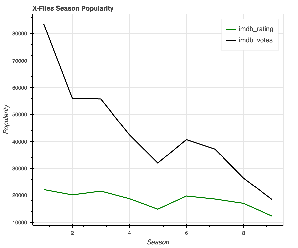
X-Files viewers seem to enjoy the first three seasons the most, with a sharp drop at season 5.
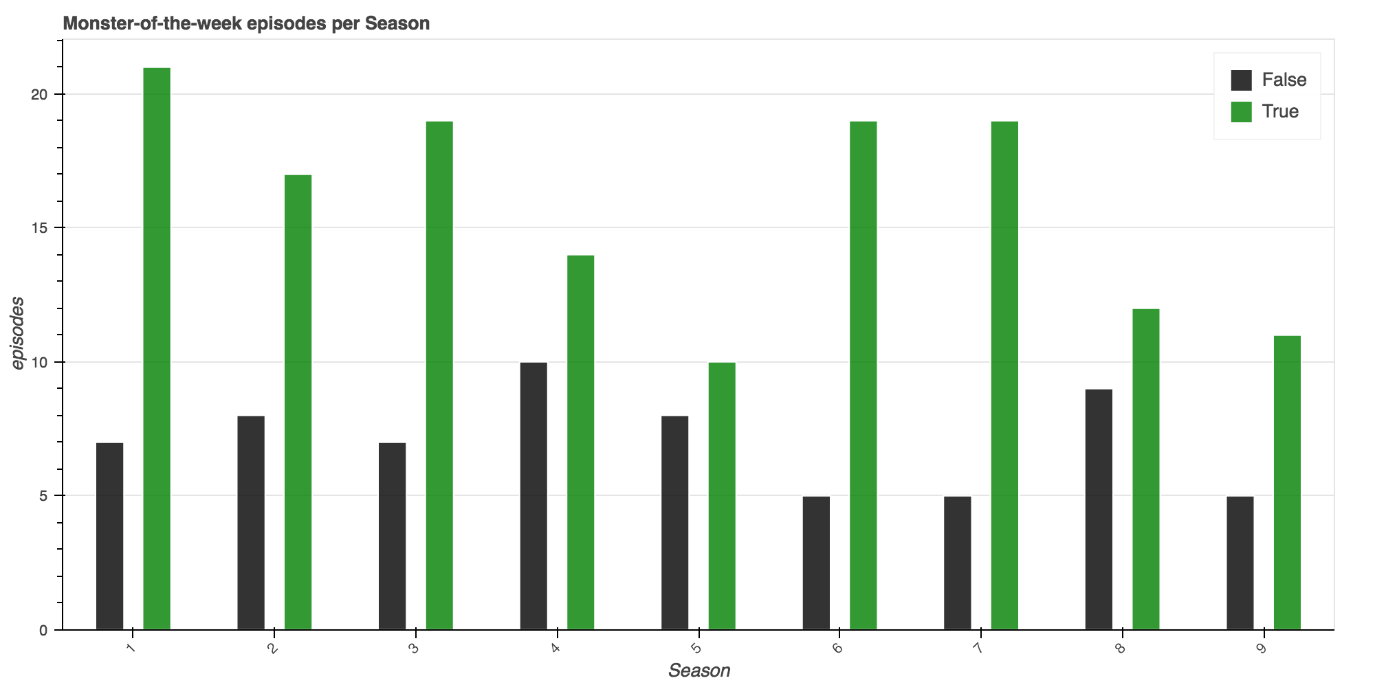
Next, I began classifying the show by the “Monster of Week” attribute I defined earlier.
# First, by season
df_monster_by_season = df.groupby(["season", "is_monster_of_the_week"]).apply(len).reset_index()

# Total monster-of-the-week
df_monster_total = df.groupby(["is_monster_of_the_week"]).agg({
    "episodeID": len,
    "imdb_rating": np.mean,
}).reset_index()
df_monster_total.columns = ["monster_of_the_week", "imdb_rating", "count"]
df_monster_total.head()
| monster_of_the_week | imdb_rating | count | |
|---|---|---|---|
| 0 | False | 8.510938 | 64 |
| 1 | True | 7.864539 | 142 |
IMBD Reviewers on average reviewed Non Monster-of-the-Week episodes ~0.65 stars higher than their counter parts.
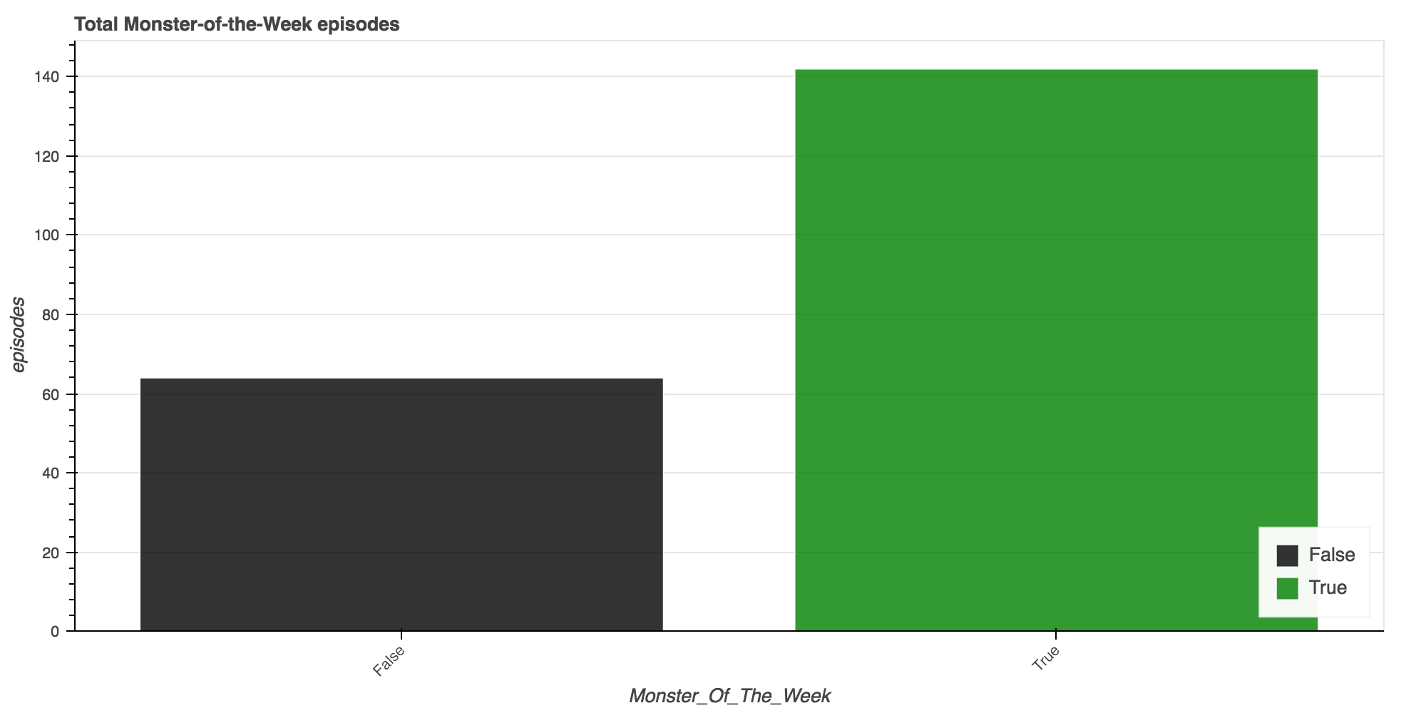
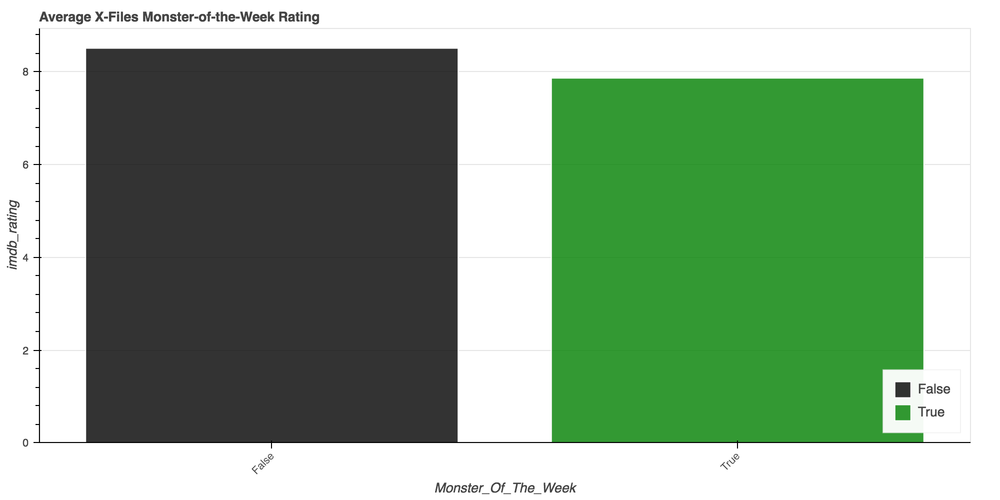
Episodes centered on the overall narrative of the show were on average received better!
Finally, I had to do a bit more cleansing with the writer data to correctly perform metrics based on a writer.
Since multiple writers can be credited on a single episode, the dataset’s records needed to be spread to a episode|writer basis.
With the writer_cleaned column stored as a list, I used the pandas apply method to append each episode|writer record to a new dataframe:
# only keeping these columns
cols = [
    "imdb_votes",
    "imdb_rating",
    "season",
    "episodeID",
]
rows = []
_ = df.apply(lambda row: [rows.append([row[c] for c in cols] + [w])
                         for w in row["writer_cleaned"]], axis=1)
df_new = pd.DataFrame(rows, columns=cols + ["writer"])
This new dataset was then aggreated to find the total number of episodes per writer and the average imdb_rating per writer.
df_writer = df_new.groupby("writer").agg({
    "episodeID": len,
    "imdb_votes": np.sum,
    "imdb_rating": np.mean,
}).reset_index()
df_writer.rename(columns={"episodeID":"episodes"}, inplace=True)
df_writer.sort("episodes", ascending=False, inplace=True)
df_writer.head()
| writer | imdb_rating | imdb_votes | episodes | |
|---|---|---|---|---|
| 5 | Chris Carter | 8.066341 | 392672.0 | 205 |
| 13 | Frank Spotnitz | 8.306818 | 68265.0 | 44 |
| 43 | Vince Gilligan | 8.425000 | 48820.0 | 28 |
| 23 | John Shiban | 7.904545 | 34321.0 | 22 |
| 17 | Howard Gordon | 7.645000 | 41683.0 | 20 |
- 👏 👏 👏 Chris Carter with 205 writing credits and an average imdb rating of 8.066341.
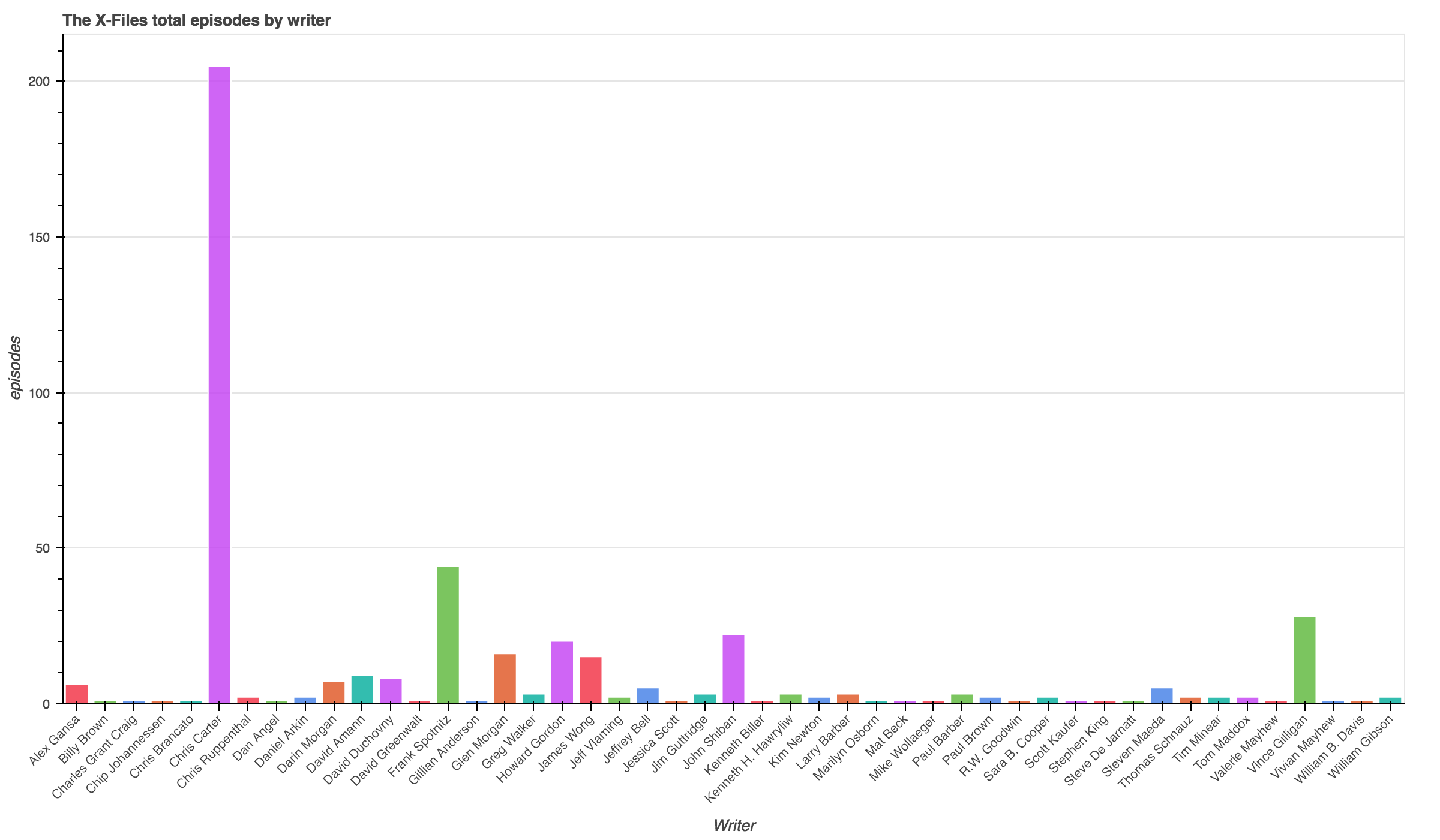
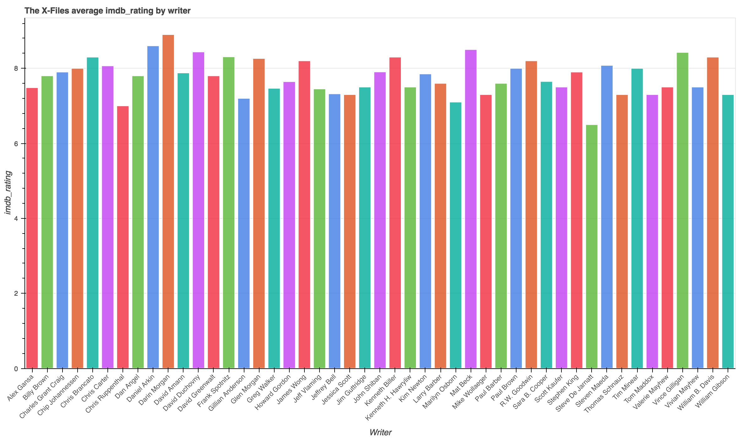
- Darin Morgan was the most well recieved writer from X-Files. He wrote 7 episodes with an average rating of 8.9000.
- Woah, Stephen King and William Gibson wrote X-Files episodes?!
The full ipython notebook with all function defintions is available here